In the world of data science, dealing with complex datasets is a common challenge. Often, these datasets don't conform to simple patterns and can't be adequately described by a single model. When faced with such data, it's essential to employ sophisticated techniques that can uncover hidden patterns and structures.

One such powerful technique is segmental least squares fitting. Instead of trying to fit a single model to the entire dataset, segmental least squares fitting breaks the data into segments and fits a separate model to each segment. This approach allows for more flexibility and accuracy in capturing the underlying trends present in the data.

To show its power, allow me to compare it against other regression methods on the Python - Past, Present, Future dataset.

On creating the Number of Users Vs. Year plot:

I have talked more about the nature of the graph in Food for thought on the data section. Furthermore I have used he metric, which is also known as Coefficient of determination.

Upon visual inspection, it's clear that the data doesn't follow a simple linear trend. However, let's start by fitting a linear model to see how well it captures the overall trend. The equation for the linear best fit is given by:

with the . The low does clarify our initial concerns about this being a subpar regression tool in this case.

this can be implemented as follows

import numpy as np
import pandas as pd
import matplotlib.pyplot as plt
from scipy.optimize import curve_fit
from sklearn.metrics import r2_score

def linear(x, m, c):
	return m * x + c

def fit_and_plot_curves(x, y):	
	try:
		params, _ = curve_fit(linear, x, y, maxfev=10000)
		y_fit = linear(x, *params)
		r2 = r2_score(y, y_fit)
		plt.plot(x, y_fit, label=f'{name}')
		print(f"fit parameters: {params}, R²={r2:.4f}")
	except (RuntimeError, ValueError, OverflowError) as e:
		print(f"Could not fit the curve: {e}")

	plt.xlabel('X')
	plt.ylabel('Y')
	plt.legend()
	plt.title('Curve Fitting')
	plt.savefig('curve_fit.svg')
	plt.close()

if __name__ = "__main__":
	# Plot the original data points	
	plt.figure(figsize=(10, 6))
	plt.scatter(x, y, color='blue', label='Data Points')

	# Read the data
	data = pd.read_csv("data/python.csv", encoding='utf-8')
	x = data["Year"].values
	y = data["Num Users"].values

	# Find the best fit
	fit_and_plot_curves(x, y)
Copy

note that we are sending in an equation of form to be fitted.

A linear model may not be sufficient to capture the nuances present in the data. Let's explore a more flexible model by fitting a polynomial. The equation for the polynomial best fit is given by:
with the , which shows a significant improvement.

As implemented in Linear best fit, we can use a similar code, but instead here we change the function to be fit .

import numpy as np
import pandas as pd
import matplotlib.pyplot as plt
from scipy.optimize import curve_fit
from sklearn.metrics import r2_score

def polynomial(x, a, b, c):
	return a * x**2 + b * x + c

def fit_and_plot_curves(x, y):	
	try:
		params, _ = curve_fit(polynomial, x, y, maxfev=10000)
		y_fit = polynomial(x, *params)
		r2 = r2_score(y, y_fit)
		plt.plot(x, y_fit, label=f'{name}')
		print(f"fit parameters: {params}, R²={r2:.4f}")
	except (RuntimeError, ValueError, OverflowError) as e:
		print(f"Could not fit the curve: {e}")

	plt.xlabel('X')
	plt.ylabel('Y')
	plt.legend()
	plt.title('Curve Fitting')
	plt.savefig('curve_fit.svg')
	plt.close()

if __name__ = "__main__":
	# Plot the original data points	
	plt.figure(figsize=(10, 6))
	plt.scatter(x, y, color='blue', label='Data Points')

	# Read the data
	data = pd.read_csv("data/python.csv", encoding='utf-8')
	x = data["Year"].values
	y = data["Num Users"].values

	# Find the best fit
	fit_and_plot_curves(x, y)
Copy

While global models like linear or polynomial fits can provide valuable insights, they may not capture local variations in the data. Segmental least squares fitting addresses this limitation by breaking the data into segments and fitting separate models to each segment.

For the Python user data, segmental least squares fitting reveals distinct segments with varying growth rates over time:

and with a , showing the best score.

For the code implementation of segmented squares, we can use dynamic programming as shown below. Here we minimize both the MSE and the number of segments that are being used.

import numpy as np
import pandas as pd
import matplotlib.pyplot as plt
import argparse

def compute_error(x, y, i, j):
    """Compute the least squares error of fitting a line to points (x[i:j], y[i:j])."""
    x_segment = x[i:j]
    y_segment = y[i:j]
    A = np.vstack([x_segment, np.ones(len(x_segment))]).T
    m, c = np.linalg.lstsq(A, y_segment, rcond=None)[0]
    y_fit = m * x_segment + c
    error = np.sum((y_segment - y_fit) ** 2)
    return error

def segmental_least_squares(x, y, max_segments):
    """Perform segmental least squares fitting using dynamic programming."""
    n = len(x)
    C = np.full((n, max_segments + 1), np.inf)
    partition = np.zeros((n, max_segments + 1), dtype=int)

    # Initialize the cost for one segment
    for i in range(n):
        C[i, 1] = compute_error(x, y, 0, i + 1)

    # Fill the dynamic programming table
    for k in range(2, max_segments + 1):
        for j in range(1, n):
            for i in range(j):
                error = compute_error(x, y, i + 1, j + 1)
                if C[i, k - 1] + error < C[j, k]:
                    C[j, k] = C[i, k - 1] + error
                    partition[j, k] = i

    # Backtrack to find the optimal segmentation
    segments = []
    current_segment = n - 1
    for k in range(max_segments, 0, -1):
        if current_segment == 0:
            break
        start_segment = partition[current_segment, k]
        segments.append((start_segment + 1, current_segment + 1))
        current_segment = start_segment

    segments.reverse()
    return segments, C[n - 1, max_segments]

def plot_segments(x, y, segments, x_label: str, y_label: str, title: str, output: str):
    """Plot the original points and the fitted segments."""
    plt.figure(figsize=(10, 6))
    plt.scatter(x, y, color='blue', label='Data Points')

    y_combined_fit = np.zeros_like(y)
    for (start, end) in segments:
        x_segment = x[start-1:end]
        y_segment = y[start-1:end]
        A = np.vstack([x_segment, np.ones(len(x_segment))]).T
        m, c = np.linalg.lstsq(A, y_segment, rcond=None)[0]
        y_fit = m * x_segment + c
        y_combined_fit[start-1:end] = y_fit
        plt.plot(x_segment, y_fit, color='red', label='Fitted Segment' if start == segments[0][0] else "")

    # Calculate combined R-squared
    ss_res_combined = np.sum((y - y_combined_fit) ** 2)
    ss_tot_combined = np.sum((y - np.mean(y)) ** 2)
    r_squared_combined = 1 - (ss_res_combined / ss_tot_combined)

    plt.xlabel(x_label)
    plt.ylabel(y_label)
    plt.title(title)
    plt.legend()
    plt.savefig(output)
    plt.close()
    print(f"Plot saved as '{output}'")
    
    return r_squared_combined

# Read points from a CSV file
def read_points_from_csv(filename: str, x_column_name: str, y_column_name: str, delimiter: str):
    data = pd.read_csv(filename, delimiter=delimiter, encoding='utf-8')
    x = data[x_column_name].values
    y = data[y_column_name].values
    return x, y

def print_equations(segments, x, y):
    """Print the equations of the fitted segments."""
    for idx, (start, end) in enumerate(segments):
        x_segment = x[start-1:end]
        y_segment = y[start-1:end]
        A = np.vstack([x_segment, np.ones(len(x_segment))]).T
        m, c = np.linalg.lstsq(A, y_segment, rcond=None)[0]
        print(f"Segment {idx+1}: y = {m:.8e} * x + {c:.8e}, for x in [{x[start-1]}, {x[end-1]}]")

if __name__ == "__main__":
	# Little arg parse magic to make the program well structured
    parser = argparse.ArgumentParser(description='Segmental Least Squares Fitting')
    parser.add_argument('filename', type=str, help='Input CSV file name')
    parser.add_argument('-x', '--x_col', type=str, default='X', help="Name of the column containing x values, default is 'X'")
    parser.add_argument('-y', '--y_col', type=str, default='Y', help="Name of the column containing y values, default is 'Y'")
    parser.add_argument('-d', '--delim', type=str, default=',', help="Delimiter used in the CSV file, default is ','")
    parser.add_argument('-m', '--max_segs', type=int, default=3, help='Maximum number of segments, default is 3')
    parser.add_argument('-t', '--title', type=str, default='Segmental Least Squares Fitting', help="Plot title, default is 'Segmental Least Squares Fitting'")
    parser.add_argument('-o', '--output', type=str, default='output.svg', help="Output file path, default is 'output.svg'")

    args = parser.parse_args()

    x, y = read_points_from_csv(args.filename, args.x_col, args.y_col, args.delim)
    segments, total_cost = segmental_least_squares(x, y, args.max_segs)
    print("Number of segments: ", len(segments))
    print("Optimal Segments:", segments)
    print("Total Cost:", total_cost)

    # Print the equations of the segments
    print_equations(segments, x, y)

    # Plot the segments and get combined R-squared
    r_squared_combined = plot_segments(x, y, segments, args.x_col, args.y_col, args.title, args.output)
    print(f"Combined R-squared: {r_squared_combined:.4f}")

Copy

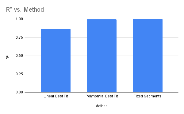
In conclusion, while segmental least squares fitting provides valuable advantages, including flexibility and accuracy, its use requires careful consideration of trade-offs between complexity and interpretability. With cautious application, data scientists can leverage this technique to extract meaningful insights from diverse datasets.

In the graph the data seems to be segmented about 1990 to 2005, then a sudden spike, after which there is a steady time increase from 2005 to around 2018, then another huge spike followed by 2020 till 2025.

I am unsure of the reason behind the same, furthermore a quick search on google trends didn't give any fruitful results:

Although we do see a sudden spike around 2022, as google altered their data collection method January 2022 onwards, we can't dismiss this to be an artifact of the same.

Thus the reason for segmentation still remains a mystery.